Exploring hyperparameter meta-loss landscapes with Jax

A common mantra of the deep learning community is to differentiate though all the things, e.g. differentiable renderer, differentiable physics, differentiable programming language[julia, dex, myia], etc. In my own research, I’ve found that, while one can often compute a gradient, it isn’t always the most useful quantity. This is especially true with “complex” loss landscapes, because the crazier the loss landscape is, the less useful local information (i.e. the gradient) is to find a global minimum. These complex loss landscape can emerge from iterative computation such as common optimization procedures for machine learning [1, 2, 3].

In this post, we’ll walk through an example showing how extraordinarily complex meta-loss landscapes can emerge from a relatively simple setting and as a result gradients of these loss landscapes become a lot less useful.

We’ll do this in a relatively new machine learning library: Jax. Jax is amazing. I’ve been using it more and more for my research and have noticed it gaining traction at Google. Despite this, very few externally have even heard about it, let alone use it. This post I also wanted to show some features that make doing this type of exploration easy.

Why Jax?

At its core, Jax provides an API nearly identical to Numpy. There is no built in neural network library (e.g. no torch.nn, or tf.keras for example, though there are many Jax NN libraries under development (flax, haiku are my favorites). Instead, one composes a set of simple operations into whatever computation is desired.

To make things fast, Jax offers a just-in-time compiler (jit) which compiles your functions to run on CPU, GPU, and TPU. This setup provides both really fast execution (Jax models are among the fastest in the recent MLPerf benchmarks), and flexibility (Jax not only does deep learning well, but has also been used for molecular dynamics simulation, and to design Stellarator – a device to contain plasma). Jax builds upon XLA, a linear algebra compiler which is responsible for taking these low graphs, and making a fast executing program.

One core concept of Jax is function transforms. One can transform some function that operates on numerical data to another function operating on similar data. For example: jax.jit is a function transform. jax.jit(f), returns a function with the same interface but that will compile it to run fast. Jax also has automatic differentiation written in this way, jax.grad(f)(x), will return the derivative of f evaluated at x.

My favorite feature of Jax is auto vectorization. Say, we want to evaluate f on not one, but multiple inputs. We could do [f(x) for x in xs], but this will execute f many times. When leveraging deep learning accelerators, this type of sequential computation can slow things down greatly. Instead we can use vmap: jax.vmap(f)(xs). What this will do is vectorize f, and then will execute a single vectorized application. Lets say f = lambda x: np.sum(x^2), defined on rank 1 arrays. The vectorized code will instead run something like np.sum(x^2, axis=1), which operates on rank 2 arrays and returns a vector. Because we are executing a smaller number of ops, on more data, we can leverage hardware a lot better.

These program transformations are composable too. One can mix and match grad’s, vmap’s, and jit’s. I can write a complex machine learning model, g, that operates on a single example, vectorizes it, and performs backprop through this auto vectorization like this:

def batch_loss(theta, xs):
   return np.mean(jax.vmap(partial(loss_fn, theta))(xs))
grad_fn = jax.jit(jax.grad(batch_loss))

dl_dtheta = grad_fn(theta, xs)

Now instead, let’s say I want to compute per example gradients. This would usually be difficult in libraries like TF or Pytorch, but in Jax it’s just the composition of function transforms in a different order.

per_example_grad_fn = jax.jit(jax.vmap(jax.grad(loss_fn)))
batch_of_dl_dtheta = per_example_grad_fn(theta, xs)

Exploring meta-loss landscapes

One of the simplest examples of meta-learning is hyperparameter search. At surface level, one might expect that changing hyperparameters results in a predictable change in the performance of optimization. In some settings, this couldn’t be more wrong. I will demonstrate one such example here on a simple 1D loss landscape.

In the process process, I will be demonstrating some cool features of Jax including: Auto vectorization (jax.vmap) and use it to visualize both inner-loss (the problem we are training to train), and outer-loss landscapes (how performance on that problem changes with hyper parameters). Gradient computation (jax.grad, jax.value_and_grad) through complex, unrolled optimization procedures Compilation (jax.jit) sprinkled around my code to greatly speed things up

For ease of reproducing, all the code is in this colab and can be run on GPU or TPU which are both available for free.

First, some imports:

import jax
import jax.numpy as jnp
from matplotlib import pylab as plt

Inner problem: A 1D optimization problem optimized with SGDM

Let’s start by defining a simple loss function we want to minimize, in this case a 1D problem. I am calling it the inner_loss. To make things interesting, lets not just use a quadratic, but instead something a little funky looking so that we have a more complex, non-convex loss:

@jax.jit
def inner_loss(x):
 return jnp.log(x**2 + 1.0 + jnp.sin(x*3)) + 1.5

We can then use auto vectorization (vmap) to visualize this loss surface.

xs = jnp.linspace(-5, 5, 100)
plt.plot(xs, jax.vmap(inner_loss)(xs))

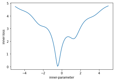
This loss has a number of interesting characteristics. It is non-convex, and has 2 minima – a global minima at approximately x=-0.5, with a value of zero, and a local minima at approximately x=1.5 with a value of about 2.

We can use SGD + momentum with a given learning rate and momentum to train this for 50 iterations. We will make use of gradient computation via jax.value_and_grad of the inner problem as well as jax.jit to speed things up.

x = -4. # initial inner parameter
v = 0.0 # initial momentum accumulator
 
lr = 0.1
mom = 0.9
 
value_and_grad_fn = jax.jit(jax.value_and_grad(inner_loss))
 
losses = []
for i in range(50):
 loss, grad = value_and_grad_fn(x)
 v= mom*v + grad
 x = x - lr * v
 losses.append(loss)
plt.plot(losses)
plt.xlabel("inner-step")
plt.ylabel("inner-loss")

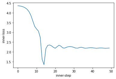
We can see we first descend into the global minima, then move out (due to momentum) to settle in the local minima.

Outer-loss: Optimization performance as a function of optimizer hyperparameters

Now, let’s explore how our inner problem training behaves as a function of momentum and learning rate. To do this, we will define an outer_loss function which, for a given set of hyperparameters, computes the mean inner-loss over the 50 step unroll. This can be considered a measurement of how “good” the learning rate and momentum are to train this inner-problem quickly and to a low loss. We can jit this /entire/ unrolled computation so it runs fast.

@jax.jit
def outer_loss(lr, mom):
 value_and_grad_fn = jax.jit(jax.value_and_grad(inner_loss))
 
 x = -4.
 v = 0.0
 losses = []
 for i in range(50):
   loss, grad = value_and_grad_fn(x)
   v= mom*v + grad
   x = x - lr * v
   losses.append(loss)
 return jnp.mean(jnp.asarray(losses))

To get a sense of this outer-loss function, we can leverage auto vectorization (jax.vmap) again, and plot the outer-loss as a function of learning rate. Here the in_axes denotes which dimensions to vectorize – in this case, add a batch dimension to argument zero (learning rate), but don’t add any to argument one (momentum).

lrs = jnp.logspace(-3, 2, 5000)
plt.semilogx(lrs, jax.jit(jax.vmap(outer_loss, in_axes=(0, None)))(lrs, 0.9), "-")
plt.ylim(-2.6, 5.0)

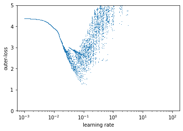
This leads to a kinda funky result. First, the loss surface is incredibly sensitive to the learning rate – much more than traditionally considered. Despite being an entirely deterministic optimization problem there appears to be noise. This means small changes in learning rate compound and produce dramatically different behaviors reminiscent of chaos.

We don’t have to stop there though, we can compose vmap and apply it twice to plot the entire outer-loss landscape. Here, we are going to parameterize the momentum via 1-log(val). This is because momentum values are usually something like 0.9, 0.99, 0.999 and so on, so to plot it makes sense to space those evenly.

lrs = jnp.logspace(-3, 2, 2000)
moms = 1. - jnp.logspace(-3, 0, 2000)
lrs, moms = jnp.meshgrid(lrs, moms)
 
img_fn = jax.vmap(jax.vmap(outer_loss))
 
plt.figure(figsize=(10,10))
img = img_fn(lrs, moms)
 
plt.imshow(img, extent=[-3, 2, 0, -3], aspect="auto", interpolation="nearest", vmax=10)
plt.xlabel("log learning rate")
plt.ylabel("log (1 - momentum)")
plt.colorbar()

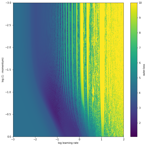
The outer-loss function continues to be kinda crazy – full of local minimum and quite high curvature. There is also this periodic behavior with learning rate, and what appears to be a low loss region that is low momentum and lower learning rate.

Outer-optimization with gradients

Now on this simple, 2D problem, to find good parameters we can simply take the min of a bunch of random trials. This doesn’t scale well to a lot of hyper parameters though and would make for a boring example. Another less common approach that people often try (to varying degrees of success) is to use gradient descent to find hyperparameters.

With Jax, this can be done relatively simply by applying jax.grad to the outer-loss function. But first, let’s define our outer-loss function that operates on a tuple of parameters (lr, mom) as opposed each as separate inputs. Second, let us change the parametrization so steps in the learning rate / momentum roughly have a similar effect regardless of the parameter location. In this case, we can do this by exponentiating the learning rate variable, and taking one minus the exponentiated momentum variable.

@jax.jit
def outer_loss(outer_params):
 log_lr, one_minus_log_mom = outer_params
 lr = jnp.power(10, log_lr)
 mom = 1.0 - jnp.power(10, one_minus_log_mom)
 x = -4.
 v = 0.0
 losses = []
 for i in range(50):
   loss, grad = value_and_grad_fn(x)
   v= mom*v + grad
   x = x - lr * v
   losses.append(loss)
 return jnp.mean(jnp.asarray(losses))

We can compute outer gradients (and the outer-loss value) with this:

outer_grad_fn = jax.jit(jax.value_and_grad(outer_loss))

And, use a minimal training loop to meta-train / outer-train. Now this training loop also clips the outer-gradients. Looking at the loss surface visualizations above, the gradients can have extremely high magnitudes. Without this clipping, outer-training quickly diverges with SGD.

outer_params = (-2., -0.5)
 
outer_params_traj = [outer_params]
 
losses = []
grads = []
alpha = 0.01
for i in range(100):
 loss, outer_grad = outer_grad_fn(outer_params)
 grads.append(outer_grad)
 outer_grad = jax.tree_map(lambda x: jnp.clip(x, -10.0, 10.0), outer_grad)
 outer_params = jax.tree_multimap(lambda a,b: a-alpha*b, outer_params, outer_grad)
 outer_params_traj.append(outer_params)
 losses.append(loss)

We can plot this trajectory on the original loss surface.

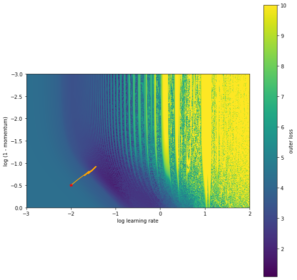
It looks like this found a local minimum as we are not moving any further. We can see evidence of this by looking at the loss surface right around the solution found. We can do this easily with jax.vmap again.

ts = jnp.linspace(-0.05, 0.05, 100)
vs = jax.jit(jax.vmap(outer_loss, in_axes=((None, 0), )))((outer_params[0], outer_params[1] + ts))
plt.plot(ts, vs, label="mom shift")
 
ts = jnp.linspace(-0.05, 0.05, 100)
vs = jax.jit(jax.vmap(outer_loss, in_axes=((0, None), )))((outer_params[0]+ts, outer_params[1]))
plt.plot(ts, vs, label="lr shift")
 
plt.ylabel("outer-loss")
plt.xlabel("shift")
plt.legend()

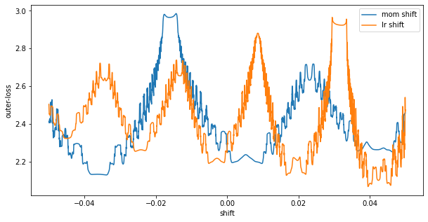
What I am showing here is shifts in learning rate centered at our final iterate. At shift=0, we see we are at what looks to be a local minimum. Moving a bit in either the learning rate or the momentum direction will increase the loss. We also see a really high curvature surface – it will be incredibly easy to get stuck in these ripples.

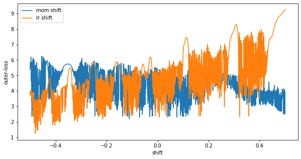
Overall, we got pretty lucky there though. The solution we found was still pretty good in the grand scheme of things. We can run this same procedure initializing the learning rate and the momentum in a more unstable regime and we will get stuck in a much worse position.

And looking at our final hyperparameters we can see that around x=0, (shift=0), the final point of our gradient based training) we are stuck in an unstable (highly sensitive to outer-parameter) region.

Outer-optimization with ES

This illustrates some of the difficulty trying to use gradient based methods to train hyperparameters. Instead of using gradients computed via backprop, we can leverage a stochastic algorithm – in this case Evolutionary Strategies. The core idea is simple, and has been written up many places before. At a high level, ES samples points around the current outer-parameter value, and moves in the direction of decreased loss. This effectively smooths out the loss surface.

To implement this, we must make use of Jax’s random number generation. Randomness is one area Jax’s design diverges from Numpy. In particular, Numpy leverages a global random number state. (np.random.RandomState also exists, which isn’t global, but still relies upon mutated state.) Instead, Jax leverages pure and stateless random number generation. One specifies a random state, the key as it is often called: key = jax.random.PRGKey(seed), and can use this key to generate deterministic, pseudo random numbers: jax.random.normal(key, ..). What this means is with the same key, two calls to jax.random.normal(key, ..) will return the same value.

To get around this, Jax implements various ways to split / generate new keys. So if one wants to generate two random numbers, one can create 2 keys: key1, key2 = jax.random.split(key, 2) then generate a number using each key.

With this, we can implement ES. In our case, I am using antithetic samples. What this means is we will sample some noise value, run the outer-function on the base parameters plus this noise, and the base parameters minus this noise. We will then compare these two values, and produce a gradient that moves in the lower loss direction.

def outer_gradient_es(outer_params, key, std):
 lr_noise, mom_noise = jax.random.normal(key, [2])*std
 outer_params_pos = (outer_params[0] + lr_noise, outer_params[1]+mom_noise)
 outer_params_neg = (outer_params[0] - lr_noise, outer_params[1]-mom_noise)
 pos_loss = outer_loss(outer_params_pos)
 neg_loss = outer_loss(outer_params_neg)
  factor = (pos_loss - neg_loss) / (2 * std**2)
 outer_grad = (lr_noise * factor, mom_noise * factor)
 return (pos_loss + neg_loss) / 2, outer_grad

Outer training looks similar to before, but now instead of using gradient we will use the above.

 std = 0.1
 loss, outer_grad = outer_gradient_es(outer_params, key1, std)
 outer_grad = jax.tree_map(lambda x: jnp.clip(x, -10.0, 10.0), outer_grad)
 outer_params = jax.tree_multimap(lambda a,b: a-alpha*b, outer_params, outer_grad)

Outer-training for a few thousand steps leads the following trajectory in the 2D space of outer-parameters:

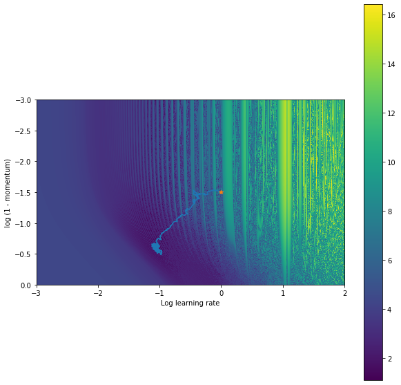
Still not perfect, but all things considered fairly good. It reaches a much better solution than the gradient based method. To make this better, we could anneal the std of ES, use smaller learning rates, use more samples for ES. Conclusion I hope this demonstrates a bit of an insight into hyperparameter loss landscapes and how care should be taken when computing gradients through unrolled optimization problems as well as a bit of why so many researchers are loving Jax. Interested in exploring any of this further? Grab a free GPU / TPU colab and give it a go – Jax is included by default. My notebook can be found here.

Acknowldgements

Thanks so much to Chip Huyen, the best writer I know, and my amazing colleagues C. Daniel Freeman and Utku Evci for feedback on this post. Thanks Mat Kelcey for the much shorter clolab + tpu snippet.

Luke Metz

Tweet Share