Deep Learning to Control my Robotic Arm
- 7 minsThis is the third installment in the chronicle of my attempt to build a robotic arm to make me tea. For the mechanical build, see here, and for the electrical and software groundwork for this post, see here.
This thing is borderline impossible to control with an Xbox controller. Not only are there too many joints, there is no notion of correcting for the forces of gravity. As such, my first plan of attack is to see if I can build some controls that make it easier to control the arm by hand – in specific, when I release the controls on my XBox controller, I would like the robot to stop moving as opposed to come crashing down. From here, the hope is that I can then do point-to-point movement and “program” it to do tasks by running through a set of predefined states. This roadmap is designed to be sample efficient. Unlike Google, I do not have an army of these arms at my disposal. This means that the more “traditional” deep reinforcement learning approaches (model-free control) are out of the question, as they are just too sample inefficient. It’s going to take a while then to get this point, but this is what I have so far.
In this post, I review the data collection and processing, discuss the forward dynamics model training, and finally, address the use of the model predictive control algorithm I employed and some initial results when applied on only 1 dimension. This post is almost entirely derived from “Model-based Reinforcement Learning with Neural Network Dynamics”, and in paper form. I highly recommend both.
Data pre-processing:
As mentioned before, I log all data that is sent (motor commands) and received (accelerometer and gyro readings). To collect some data, I ran the robot with random-ish movements (generated by me and an XBox controller) for roughly 10 min. These are saved to ndjson files on disk. Importantly, data are received at specific instances of time, and are at different frequencies and not aligned. I resample the data to correct for this at some fixed rate. For this first test, I am resampling at 100 Hertz using the wonderful np.interp.
Forward Modeling:
My forward dynamics model takes the current sensor readings (the state, in reinforcement learning speak), and the control commands (the actions), and predicts the next sensor 1/100th of a second later. To complicate things, these commands do not happen instantly. This is partially attributable to the software side of things, and partially to the mechanical system itself – a motor cannot simply go from off to full power instantaneously. As such, this model must take into account this hidden information when making predictions. Technically speaking, the system I am modeling is a POMDP.
The model I chose to work with first is a LSTM, as it’s capable of modeling these hidden states naturally.
I used a 64 unit hidden state model, with a linear layer transforming the output into the predicted actions. As done in Nagabandi et. al., instead of predicting the next state, the model predicts the difference from the current state to the next state. Additionally, to make the predictions of a sane scale (motors don’t move all that much in 1/100th of a step), I normalized the differences to unit mean and variance by estimating the mean and variance of the deltas over the training data.
The full update can be written as \(s_{t+1} = s_t + p(s_t, a_t; \theta) \sigma^2 + \mu\) where \(p(\cdot)\) is a normalized sample, and \(\sigma^2\) and \(\mu\) are the normalizing variance and mean of the training data respectively. Additionally, unlike the work from Nagabandi et al., I chose to use a stochastic model instead of a deterministic one. If you do the math, their model can also be written down exactly as optimizing log likelihood under a normal distribution with a fixed variance, but I figured I would just model it explicitly as such, and learn the normal distributions variance while I am at it. Instead of the mean squared error loss, I minimize the negative log likelihood of the next state given all the current \((x_t, a_t)\) and past information \(h_t\).
\[L = -\text{log}(p(x_t+1 | x_t, h_t, a_t; \theta))\]For training data, I take 10 second random slices, and run them through the model (with teacher forcing) with a batch size of 32. Additionally, I have a “test set” – a set of data collected after turning off and on the robot– to get at least some measure of over fitting. I train with the Adam optimizer and early stopped when the test loss stopped improving (in this case, 30 min).
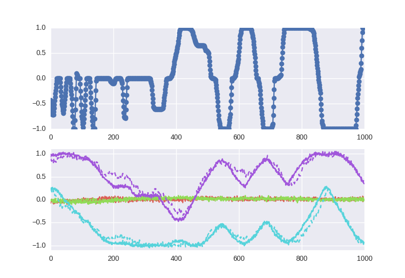
To gain a quick sanity check of the model, I recreated a plot from Nagabandi et al., where they run the forward dynamics model for some amount of time and compare it to the ground truth data. Despite a seemingly horribly high loss, the predicted trajectories on test data appear reasonably good, at least good enough to test it for control.
Model Predictive Control Policy:
With the model done, I next turned to actually using it. A forward dynamics model alone is not enough to do control. One needs to convert this into some form of policy. For this, I used model predictive control. Despite the fancy Wikipedia page, I believe this is actually a rather simple procedure – first, “plan” somehow into the future using the current model, then perform only the first step of this plan. This will bring you to a new state in which another round of planning occurs.
As my first control task, I tried simply to return to a given state. To keep things simple, instead of “planning” I picked a few fixed action sets. In my case, setting the motor on for 3 seconds each at one of the following powers: 1.0, 0.5, 0.0, -0.5, -1.0. I used these “plans” and did rollouts under the model. The best plan was the action sequence that put the final state closest to the target position. This is totally not ideal, and will not even converge in a lot of cases, but it’s a start! I tried this on the robot, and it almost kinda works, but oscillates around the correct solution.
Why does it oscillate? I am not entirely sure, but I am fairly confident that it has to do with the control frequency and latency in the model. First, I am issuing the command AFTER the model has finished making predictions. This means that while the model is churning away, the previous command is still executing on the robot and modifying the current state. This type of time delay can (and seems to) lead to oscillations. To validate this, I increased the amount of compute, and the oscillations got bigger.
Next up:
I have a few ideas as to how to remedy this time delay issue – I think it’s enough to set a fixed control frequency (say, 10 Hertz), and in the planning stage, plan as if the previous action was being executed for this amount of time. Doing this, however, will require another few weekends. I am going to put this effort on hold for now though and shift focus to a second, more powerful version of the mechanical design. Update soon!
